4 Hydrodynamics
Hydrodynamics, a branch of fluid mechanics, studies the motion of liquids and the forces acting on them. Unlike aerodynamics, which concerns compressible gases such as air, hydrodynamics primarily deals with incompressible fluids like water. It is based on classical physics principles, including Newton’s laws of motion, the conservation of mass and momentum. These principles are used to describe the velocity, pressure and viscosity of a fluid in motion.
4.1 Volume Flow Rate
Volume rate of flow refers to the rate at which a fluid volume passes a given section in a flow stream. Volume rate of flow may also be referred to as capacity of flow, flow rate or discharge. It is generally given in units of volume per unit of time, cubic meters per second (m3/s) or liters per second (L/s).
Consider an ideal fluid flow in a pipe of cross-section ‘A’ (m2). For an ideal fluid all the particles move to the right with a velocity of ‘C’ (m/s). As the fluid flow to the right with a velocity of C m/s, ‘C’ m of fluid pass section 1 every second. i.e. the volume of fluid passing section-1 every second is A x C.
\[ \dot{v} = A \cdot C \]
Where:
\(\dot{v}\): Volume flow rate, \(\mathrm{m^3/s}\)
\(A\): Cross-sectional area of the flow, \(\mathrm{m^2}\)
\(C\): Mean (average) velocity of the fluid, \(\mathrm{m/s}\)
Consider a real fluid flowing in the same pipe. Here particle velocity will be a variable across the flow stream.
If the mean velocity cm of all the fluid particles could be found, then similar to the ideal fluid.
\[ Volume\ flow = area\ x\ mean\ velocity \]
Unless otherwise indicated, the velocity of flow is understood to refer to the average or mean velocity of all the particles in a flowing fluid.
4.2 Mass Flow Rate
Mass flow rate refers to the rate at which a fluid mass passes a given section in a flow stream. It is given in units of mass per unit of time, kilogram per second (kg/s). Mass flow rate is easily calculated from volume flow rate as follows.
\[ \dot{m} = \rho \cdot \dot v \]
Where:
\(\dot{m}\): mass flow rate, \(\mathrm{kg/s}\)
\(\rho\): density, \(\mathrm{kg/m^3}\)
\(\dot{v}\): volume flow, \(\mathrm{m^3/s}\)
Or
\[ \dot{m} = \rho \cdot A \cdot C \]
Where:
\(\dot{m}\): mass flow rate, \(\mathrm{kg/s}\)
\(\rho\): density, \(\mathrm{kg/m^3}\)
\(A\): Cross-sectional area of the flow, \(\mathrm{m^2}\)
\(C\): Mean (average) velocity of the fluid, \(\mathrm{m/s}\)
Example 4.1 Oil of relative density 0.9 flows at full bore through a pipe with an internal diameter of 75 mm at a velocity of 1.2 m/s. Calculate the volume flow rate in cubic metres per second and the mass flow rate in tonnes per hour.
"""
Pipe Flow Rate Calculator for Oil

Determines the volumetric and mass flow rates in a pipe carrying oil,
given the internal diameter, fluid velocity, and relative density.
"""

import math

# ==============================
# INPUT PARAMETERS
# ==============================

pipe_internal_diameter_mm = 75.0  # Pipe internal diameter in millimeters
oil_velocity_m_per_s = 1.2  # Average velocity of oil in m/s
oil_relative_density = 0.9  # Specific gravity of oil (relative to water)
water_density_kg_per_m3 = 1000.0  # Density of water in kg/m³

# ==============================
# UNIT CONVERSIONS AND GEOMETRY
# ==============================

# Convert pipe diameter from millimeters to meters
pipe_internal_diameter_m = pipe_internal_diameter_mm / 1000.0

# Calculate pipe radius
pipe_radius_m = pipe_internal_diameter_m / 2.0

# Calculate cross-sectional area of the pipe (circular)
pipe_cross_sectional_area_m2 = math.pi * pipe_radius_m**2

# ==============================
# FLOW RATE CALCULATIONS
# ==============================

# Calculate volumetric flow rate using Q = A · v
volumetric_flow_rate_m3_per_s = pipe_cross_sectional_area_m2 * oil_velocity_m_per_s

# Calculate oil density from relative density
oil_density_kg_per_m3 = oil_relative_density * water_density_kg_per_m3

# Calculate mass flow rate using ṁ = ρ · Q
mass_flow_rate_kg_per_s = oil_density_kg_per_m3 * volumetric_flow_rate_m3_per_s

# Convert mass flow rate to tonnes per hour
mass_flow_rate_tonnes_per_hour = mass_flow_rate_kg_per_s * 3600 / 1000

# ==============================
# OUTPUT RESULTS
# ==============================

print("Pipe Flow Analysis Results:")
print(f"  Volumetric flow rate : {volumetric_flow_rate_m3_per_s:.4f} m³/s")
print(f"  Mass flow rate       : {mass_flow_rate_tonnes_per_hour:.4f} " f"tonnes/hour")
4.3 Discharge Through an Orifice
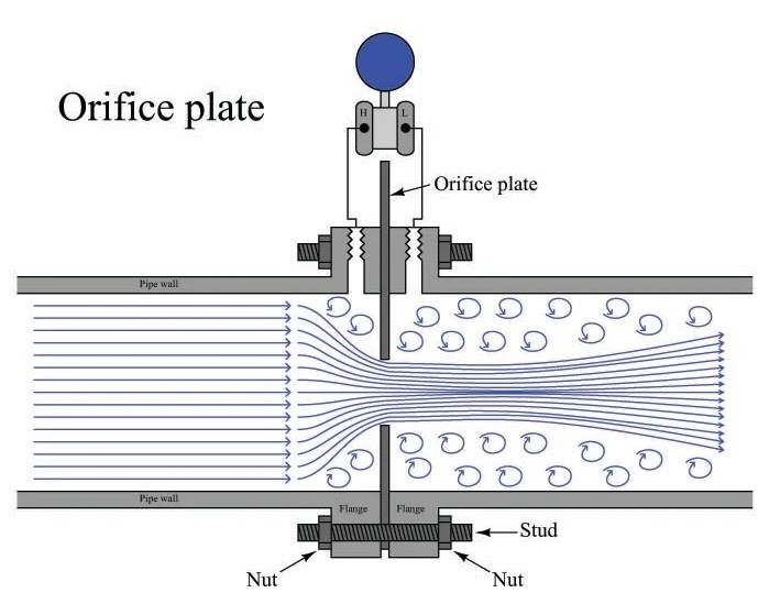
When water discharges through an orifice (Figure 4.1) in the side of a tank, the potential energy associated with the height of the water surface above the orifice is converted into kinetic energy of the efflux.
This yields the theoretical velocity of the jet: \[ C = \sqrt{2gh} \] where \(g\) is the acceleration due to gravity and \(h\) is the height of the water surface above the orifice.
The theoretical volume flow rate is then: \[ \dot{v}_{\text{theoretical}} = A C = A \sqrt{2gh} \] where \(A\) is the area of the orifice.
Due to viscous effects, the actual velocity is less than the theoretical value. The coefficient of velocity, \(C_v\), is defined as the ratio of actual velocity to theoretical velocity. Thus, the velocity-corrected flow rate is: \[ \dot{v}_{\text{velocity-corrected}} = C_v A \sqrt{2gh} \]
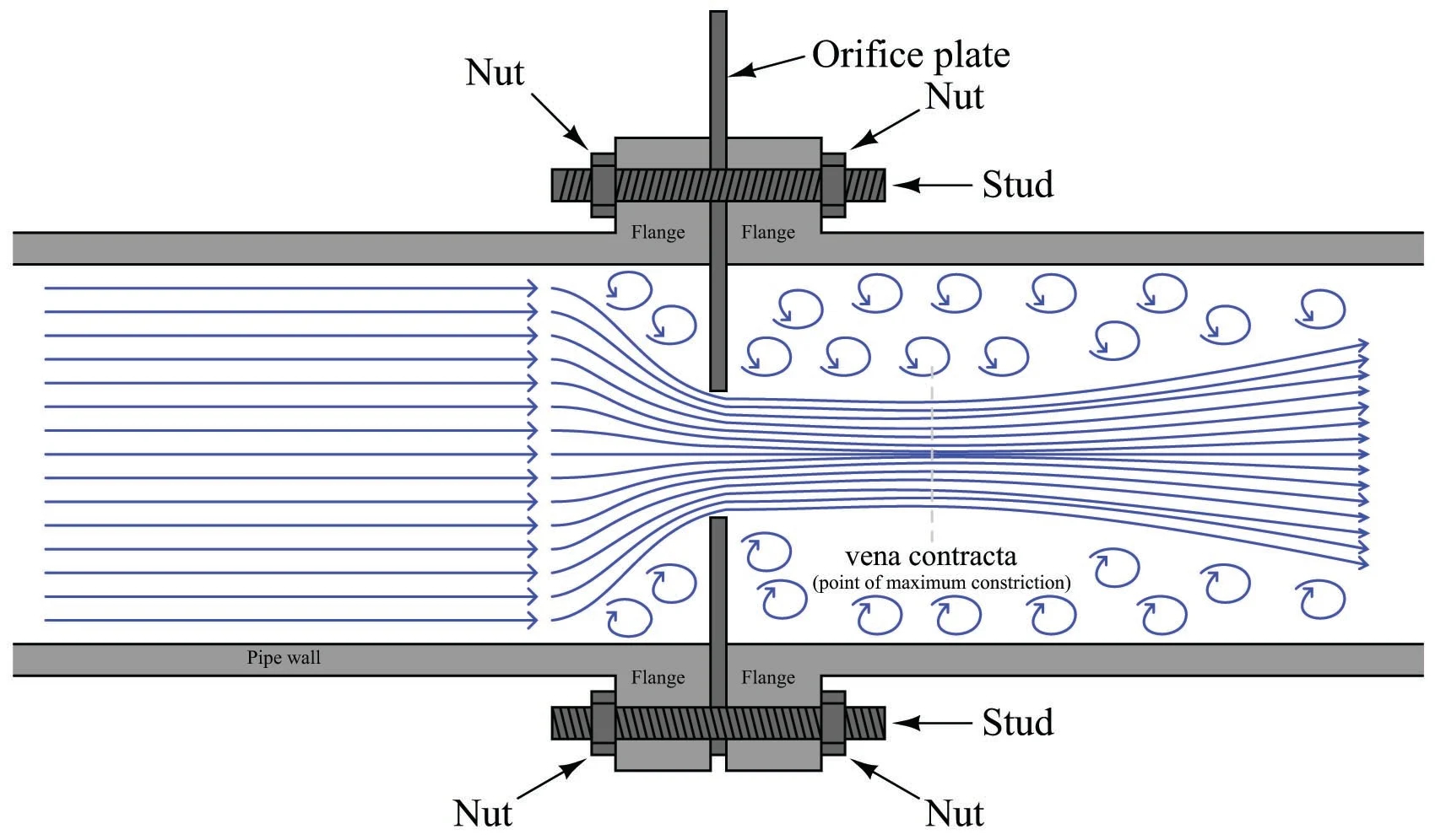
Downstream of a sharp-edged orifice, the jet contracts due to streamline curvature, forming a vena contracta (Figure 4.2). The vena contracta refers to the narrowest cross-section of a fluid jet shortly downstream of an orifice or nozzle, where the streamlines converge, resulting in the smallest area, maximum velocity, and minimum pressure.
The coefficient of contraction, \(C_A\), is the ratio of the jet area at the vena contracta to the orifice area: \[ A_{\text{jet}} = C_A A \]
The actual volume flow rate therefore becomes: \[ \dot{v}_{\text{actual}} = C_A A \cdot C_v \sqrt{2gh} \]
The coefficient of discharge, \(C_d\), is the ratio of the actual volume flow rate to the theoretical volume flow rate: \[ C_d = C_A \cdot C_v \]
Consequently, \[ \dot{v}_{\text{actual}} = C_d A \sqrt{2gh} \]
Example 4.2 Water escapes through a hole 20 mm in diameter in the side of a tank, with a water head of 3 m above the hole. Given a coefficient of velocity of 0.97 and a coefficient of reduction of area of 0.64, calculate (i) the velocity of the water jet as it exits the hole and (ii) the quantity of water escaping tonne per hour.
"""
Orifice Flow Calculator

Calculates the actual velocity and discharge rate of water escaping
through an orifice under a given head. Uses coefficient of velocity (Cv)
and coefficient of area (Ca) to account for real flow conditions.
"""

import math

# ================================
# INPUT PARAMETERS
# ================================

orifice_diameter_mm = 20  # Orifice diameter in millimeters
head_above_orifice_m = 3  # Height of water above orifice in meters
coefficient_of_velocity = 0.97  # Cv (accounts for velocity reduction)
coefficient_of_area = 0.64  # Ca (accounts for vena contracta)
gravitational_acceleration_m_per_s2 = 9.81  # Acceleration due to gravity
water_density_kg_per_m3 = 1000  # Density of water in kg/m³

# ================================
# UNIT CONVERSIONS AND GEOMETRY
# ================================

# Convert orifice diameter from millimeters to meters
orifice_diameter_m = orifice_diameter_mm / 1000

# Calculate orifice radius
orifice_radius_m = orifice_diameter_m / 2

# Calculate cross-sectional area of orifice
orifice_area_m2 = math.pi * orifice_radius_m**2

# ================================
# VELOCITY CALCULATIONS
# ================================

# Calculate theoretical velocity using Torricelli's theorem: v = √(2gh)
theoretical_velocity_m_per_s = math.sqrt(
    2 * gravitational_acceleration_m_per_s2 * head_above_orifice_m
)

# Calculate actual velocity accounting for friction losses
actual_velocity_m_per_s = coefficient_of_velocity * theoretical_velocity_m_per_s

# ================================
# FLOW RATE CALCULATIONS
# ================================

# Calculate actual volumetric flow rate: Q = Ca · A · v
# (Ca accounts for contraction of jet at vena contracta)
volumetric_flow_rate_m3_per_s = (
    coefficient_of_area * orifice_area_m2 * actual_velocity_m_per_s
)

# Calculate mass flow rate: ṁ = ρ · Q
mass_flow_rate_kg_per_s = water_density_kg_per_m3 * volumetric_flow_rate_m3_per_s

# Convert mass flow rate to per-hour basis
mass_flow_rate_kg_per_hour = mass_flow_rate_kg_per_s * 3600

# Convert mass flow rate to tonnes per hour
mass_flow_rate_tonnes_per_hour = mass_flow_rate_kg_per_hour / 1000

# ================================
# OUTPUT RESULTS
# ================================

print(f"(i) Actual velocity of the water jet: " f"{actual_velocity_m_per_s:.3f} m/s")
print("\n(ii) Quantity of water escaping per hour:")
print(f"    Volume flow rate: {volumetric_flow_rate_m3_per_s:.6f} m³/s")
print(f"    Mass flow rate: {mass_flow_rate_kg_per_s:.4f} kg/s")
print(f"    Mass per hour: {mass_flow_rate_kg_per_hour:.4f} kg/hour")
print(f"    Mass per hour: {mass_flow_rate_tonnes_per_hour:.4f} tonnes/hour")
4.4 Continuity Equation
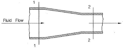
Continuous flow exists in a flow system when the mass flow rate is constant throughout the system as shown in Figure 4.3. If in the diagram below, the mass flow rate at 1 is equal to that at 2, then continuity exists.
Since \(\dot{m_1} = \dot{m_2}\), therefore
\[ \rho_1 \cdot A_1 \cdot C_1= \rho_2 \cdot A_2 \cdot C_2 \]
If the fluid is incompressible (most liquids), then density will remain constant (\(\rho_1=\rho_2\)) and the above equations may be written as:
\[ A_1 \cdot C_1= A_2 \cdot C_2 \] Or
\[ \dot{v_1}= \dot{v_2} \]
That is, the volume flow rate is constant for an incompressible fluid.
Example 4.3 A pipe decreases in diameter from 300 mm to 200 mm. Water flows from the larger to the smaller pipe at a constant rate of 18.4 kL/min. Calculate the mass flow rate and the velocities in the larger and smaller pipe.
"""
Pipe Flow Velocity Calculator

Calculates the mass flow rate and velocities in pipes of different
diameters carrying water at a constant volumetric flow rate. Uses
continuity equation to determine flow velocities.
"""

import math

# ==================================
# INPUT PARAMETERS
# ==================================

volumetric_flow_rate_kl_per_min = 18.4  # Flow rate in kiloliters/min
large_pipe_diameter_mm = 300  # Diameter of larger pipe in millimeters
small_pipe_diameter_mm = 200  # Diameter of smaller pipe in millimeters
water_density_kg_per_m3 = 1000  # Density of water in kg/m³

# ==================================
# UNIT CONVERSIONS
# ==================================

# Convert volumetric flow rate from kL/min to m³/s
# (1 kL = 1 m³, and 1 min = 60 s)
volumetric_flow_rate_m3_per_s = volumetric_flow_rate_kl_per_min / 60

# Convert pipe diameters from millimeters to meters
large_pipe_diameter_m = large_pipe_diameter_mm / 1000
small_pipe_diameter_m = small_pipe_diameter_mm / 1000

# Calculate pipe radii
large_pipe_radius_m = large_pipe_diameter_m / 2
small_pipe_radius_m = small_pipe_diameter_m / 2

# ==================================
# CROSS-SECTIONAL AREA CALCULATIONS
# ==================================

# Calculate cross-sectional area of larger pipe
large_pipe_area_m2 = math.pi * large_pipe_radius_m**2

# Calculate cross-sectional area of smaller pipe
small_pipe_area_m2 = math.pi * small_pipe_radius_m**2

# ==================================
# VELOCITY CALCULATIONS
# ==================================

# Calculate velocity in larger pipe using continuity equation: v = Q / A
velocity_large_pipe_m_per_s = volumetric_flow_rate_m3_per_s / large_pipe_area_m2

# Calculate velocity in smaller pipe using continuity equation: v = Q / A
velocity_small_pipe_m_per_s = volumetric_flow_rate_m3_per_s / small_pipe_area_m2

# ==================================
# MASS FLOW RATE CALCULATION
# ==================================

# Calculate mass flow rate using ṁ = ρ · Q
mass_flow_rate_kg_per_s = water_density_kg_per_m3 * volumetric_flow_rate_m3_per_s

# ==================================
# OUTPUT RESULTS
# ==================================

print(f"Mass flow rate: {mass_flow_rate_kg_per_s:.4f} kg/s")
print(
    f"Velocity in larger pipe ({large_pipe_diameter_mm} mm): "
    f"{velocity_large_pipe_m_per_s:.4f} m/s"
)
print(
    f"Velocity in smaller pipe ({small_pipe_diameter_mm} mm): "
    f"{velocity_small_pipe_m_per_s:.4f} m/s"
)
4.5 The Energy Equation for an Ideal Fluid
The steady flow equation is developed from the Law of Conservation of Energy. If there are no energy losses or energy additions in a flow system, then the total energy of a flowing fluid will remain constant.
A flowing fluid may lose energy as a result of fluid friction, heat energy transfer and fluid motors. For an ideal fluid, frictional losses are equal to zero. Energy may be added to a fluid via a pump or heat energy addition.
The total energy possessed by a flowing fluid consists of:
- internal energy
- potential energy
- kinetic energy and
- pressure energy (flow energy).
Generally in fluid mechanics the change in internal energy is considered to be negligible. Heat energy transfers are usually not considered in fluid mechanics and the frictional heat developed by a flowing fluid is relatively small. Therefore, the internal energy term is omitted from the energy balance.
Consider the flow system shown in Figure 4.4. For this system, assume:
- an ideal fluid
- that there are no energy losses or additions and
- steady flow conditions exist.

From the Law of Conservation of Energy:
The Total Energy at section 1 = The Total Energy at section 2
\[ mZ_1g+\frac{m C_1^2}{2}+mP_1v_1=mZ_2g+\frac{m C_2^2}{2}+mP_2v_2 \]
Dividing through by \(mg\):
\[ \frac{mZ_1g}{mg}+\frac{m C_1^2}{2mg}+\frac{mP_1v_1}{mg}=\frac{mZ_2g}{mg}+\frac{m C_2^2}{2mg}+\frac{mP_2v_2}{mg} \]
Therefore
\[ Z_1+\frac{C_1^2}{2g}+\frac{P_1v_1}{g}=Z_2+\frac{C_2^2}{2g}+\frac{P_2v_2}{g} \]
In fluid mechanics density (\(\rho\)) is generally used in preference to specific volume, i.e. \(v=\frac{1}{\rho}\) Therefore:
\[ Z_1+\frac{C_1^2}{2g}+\frac{P_1}{g\rho_1}=Z_2+\frac{C_2^2}{2g}+\frac{P_2}{g\rho_2} \]
In fluid mechanics, specific weight represents the force exerted by gravity on a unit volume of a fluid. For this reason, units are expressed as force per unit volume (e.g., \(N/m^3\))
Specific weight is given \(\gamma = g\rho\)
Where:
\(\gamma\): specific weight, \(\mathrm{N/m^3}\)
\(g\): gravitational acceleration, \(\mathrm{m/s^2}\)
\(\rho\): density, \(\mathrm{kg/m^3}\)
\[ Z_1+\frac{C_1^2}{2g}+\frac{P_1}{\gamma_1}=Z_2+\frac{C_2^2}{2g}+\frac{P_2}{\gamma_2} \]
Each term has units of m, therefore:
Potential energy \(Z\) is known as the elevation head.
Kinetic energy \(\frac{c^2}{2g}\) is known as the velocity head.
Pressure energy \(\frac{P}{\gamma}\) is known as the pressure head.
Similarly, the total energy of a flowing fluid is known as the total head (H).
\[ Total\ Head= Elevation\ Head + Velocity\ Head + Pressure\ Head \] \[ H=Z+\frac{C^2}{2g}+\frac{P}{\gamma} \]
The total head (H) will be a constant throughout a flow system if:
frictional losses (head loss) are equal to zero
work energy is not added by a pump (pump head) or removed by a motor.
Example 4.4 Consider a simple flow system consisting of a varying cross-section pipe. Water flows through this system at a rate of 2000 L/min. As the pipe increases in elevation from 30 m to 36 m it decreases in diameter from 10 cm to 3.0 cm. If the pressure is 6.5 MPa at the 30 m elevation, what is the pressure at 36 m?
"""
Energy Equation Pressure Calculator

Calculates the pressure at a higher elevation in a pipe using the energy
equation. Accounts for changes in velocity, elevation, and pressure between
two sections of a pipe carrying water.
"""

import math

# ===========================================
# INPUT PARAMETERS
# ===========================================

volumetric_flow_rate_l_per_min = 2000.0  # Flow rate in liters per minute
diameter_lower_section_m = 0.10  # Pipe diameter at lower section in meters
diameter_upper_section_m = 0.03  # Pipe diameter at upper section in meters
elevation_lower_section_m = 30.0  # Elevation at lower section in meters
elevation_upper_section_m = 36.0  # Elevation at upper section in meters
pressure_lower_section_pa = 6.5e6  # Pressure at lower section in Pascals
water_density_kg_per_m3 = 1000.0  # Density of water in kg/m³
gravitational_acceleration_m_per_s2 = 9.81  # Acceleration due to gravity

# ===========================================
# UNIT CONVERSIONS
# ===========================================

# Convert volumetric flow rate from L/min to m³/s
# (1 L = 0.001 m³, 1 min = 60 s)
volumetric_flow_rate_m3_per_s = volumetric_flow_rate_l_per_min / 60000.0

# ===========================================
# CROSS-SECTIONAL AREA CALCULATIONS
# ===========================================

# Calculate cross-sectional area at lower section
area_lower_section_m2 = math.pi * (diameter_lower_section_m / 2.0) ** 2

# Calculate cross-sectional area at upper section
area_upper_section_m2 = math.pi * (diameter_upper_section_m / 2.0) ** 2

# ===========================================
# VELOCITY CALCULATIONS
# ===========================================

# Calculate velocity at lower section using continuity equation: v = Q / A
velocity_lower_section_m_per_s = volumetric_flow_rate_m3_per_s / area_lower_section_m2

# Calculate velocity at upper section using continuity equation: v = Q / A
velocity_upper_section_m_per_s = volumetric_flow_rate_m3_per_s / area_upper_section_m2

# ===========================================
# PRESSURE CALCULATION USING ENERGY EQUATION
# ===========================================

# Apply the energy equation between lower and upper sections:
# P₁ + ½ρv₁² + ρgz₁ = P₂ + ½ρv₂² + ρgz₂
# Solving for P₂:
# P₂ = P₁ + ½ρ(v₁² - v₂²) + ρg(z₁ - z₂)

pressure_upper_section_pa = (
    pressure_lower_section_pa
    + 0.5
    * water_density_kg_per_m3
    * (velocity_lower_section_m_per_s**2 - velocity_upper_section_m_per_s**2)
    + water_density_kg_per_m3
    * gravitational_acceleration_m_per_s2
    * (elevation_lower_section_m - elevation_upper_section_m)
)

# Convert pressure to MPa for output
pressure_upper_section_mpa = pressure_upper_section_pa / 1e6

# ===========================================
# OUTPUT RESULTS
# ===========================================

print(f"Flow rate: {volumetric_flow_rate_m3_per_s:.5f} m³/s")
print(f"Area 1: {area_lower_section_m2:.6f} m²")
print(f"Area 2: {area_upper_section_m2:.6f} m²")
print(f"Velocity 1: {velocity_lower_section_m_per_s:.4f} m/s")
print(f"Velocity 2: {velocity_upper_section_m_per_s:.4f} m/s")
print(
    f"Pressure at {elevation_upper_section_m} m elevation: "
    f"{pressure_upper_section_mpa:.4f} MPa"
)
4.6 Bernoulli’s Equation
The Bernoulli’s equation between two points in a fluid flow is given by:
\[ P_1 + \frac{1}{2} \rho C_1^2 + \rho g h_1 = P_2 + \frac{1}{2} \rho C_2^2 + \rho g h_2 \]
Where:
\(P_1\) and \(P_2\) are the pressures at points 1 and 2, respectively.
\(\rho\) is the density of the fluid.
\(C_1\) and \(C_2\) are the velocities of the fluid at points 1 and 2, respectively.
\(g\) is the acceleration due to gravity.
\(h_1\) and \(h_2\) are the heights of the fluid at points 1 and 2, respectively.
4.7 Venturi Meter
A venturi meter (Figure 4.5) measures liquid flow rates in pipelines. The device features a pipe section that narrows in the middle (called the throat) and widens at both ends, as shown below:

When the entrance and throat areas are known, and the pressure readings (or pressure difference) at these points are measured, Bernoulli’s equation can be used to calculate the liquid velocity and flow rate. Typically, a venturi meter is installed horizontally in the pipeline, which simplifies calculations since there is no elevation difference between points (Z1 = Z2), thus eliminating the height terms.
Example 4.5 A horizontal venturi meter has an inlet diameter of 450 mm and a throat diameter of 225 mm. The pressure difference between these two points is equivalent to 381 mm of water. Given the density of fresh water is 1000 kg/m³, calculate the mass flow rate through the meter.
"""
Venturi Meter Flow Calculator

Calculates the flow rate through a Venturi meter using Bernoulli's
equation. Determines throat velocity and volumetric/mass flow rates
from the pressure differential between inlet and throat sections.
"""

import math

# ===============================================
# INPUT PARAMETERS
# ===============================================

inlet_diameter_m = 0.450  # Inlet diameter in meters
throat_diameter_m = 0.225  # Throat diameter in meters
pressure_head_difference_m = 0.381  # Pressure head difference in meters
gravitational_acceleration_m_per_s2 = 9.81  # Acceleration due to gravity
water_density_kg_per_m3 = 1000  # Density of water in kg/m³

# ===============================================
# CROSS-SECTIONAL AREA CALCULATIONS
# ===============================================

# Calculate cross-sectional area at inlet
inlet_area_m2 = math.pi * (inlet_diameter_m / 2) ** 2

# Calculate cross-sectional area at throat
throat_area_m2 = math.pi * (throat_diameter_m / 2) ** 2

# ===============================================
# VELOCITY CALCULATION USING BERNOULLI'S EQUATION
# ===============================================

# Compute the squared area ratio (A_throat / A_inlet)²
area_ratio_squared = (throat_area_m2 / inlet_area_m2) ** 2

# Calculate throat velocity using Bernoulli's equation for a Venturi meter:
# c₂ = √[2gh / (1 - (A₂/A₁)²)]
# where h is the pressure head difference
throat_velocity_m_per_s = math.sqrt(
    (2 * gravitational_acceleration_m_per_s2 * pressure_head_difference_m)
    / (1 - area_ratio_squared)
)

# ===============================================
# FLOW RATE CALCULATIONS
# ===============================================

# Calculate volumetric flow rate using Q = A · v at throat section
volumetric_flow_rate_m3_per_s = throat_area_m2 * throat_velocity_m_per_s

# Calculate mass flow rate using ṁ = ρ · Q
mass_flow_rate_kg_per_s = water_density_kg_per_m3 * volumetric_flow_rate_m3_per_s

# ===============================================
# OUTPUT RESULTS
# ===============================================

print(f"Entrance area: {inlet_area_m2:.6f} m²")
print(f"Throat area: {throat_area_m2:.6f} m²")
print(f"Throat velocity: {throat_velocity_m_per_s:.4f} m/s")
print(f"Volumetric flow rate: {volumetric_flow_rate_m3_per_s:.4f} m³/s")
print(f"Mass flow rate: {mass_flow_rate_kg_per_s:.4f} kg/s")
Example 4.6 A 300 mm diameter pipe has a venturi meter with a throat diameter of 100 mm. A U-tube gauge filled with water and mercury measures a pressure head difference of 250 mm between the inlet and throat. The meter coefficient is 0.95. Using the density of water (1000 kg/m³), calculate the discharge rate through the pipe in m³/s.
"""
Venturi Meter with Mercury Manometer Calculator

Calculates the actual discharge through a Venturi meter using a mercury
manometer to measure pressure difference. Accounts for the coefficient
of discharge and converts mercury column height to equivalent water head.
"""

import math

# ==================================
# INPUT PARAMETERS
# ==================================

inlet_diameter_m = 0.3  # Inlet diameter in meters
throat_diameter_m = 0.1  # Throat diameter in meters
coefficient_of_discharge = 0.95  # Discharge coefficient (dimensionless)
mercury_column_height_m = 0.250  # Manometer reading in meters of mercury
mercury_specific_gravity = 13.6  # Specific gravity of mercury (water = 1)
gravitational_acceleration_m_per_s2 = 9.81  # Acceleration due to gravity

# ==================================
# CROSS-SECTIONAL AREA CALCULATIONS
# ==================================

# Calculate cross-sectional area at inlet
inlet_area_m2 = math.pi * (inlet_diameter_m**2) / 4

# Calculate cross-sectional area at throat
throat_area_m2 = math.pi * (throat_diameter_m**2) / 4

# ==================================
# EQUIVALENT WATER HEAD CALCULATION
# ==================================

# Convert mercury column height to equivalent water head
# The pressure difference measured by mercury must be converted to
# water equivalent by accounting for the density difference:
# h_water = h_mercury × (SG_mercury - 1)
equivalent_water_head_m = mercury_column_height_m * (mercury_specific_gravity - 1)

# ==================================
# DIAMETER RATIO CALCULATION
# ==================================

# Calculate diameter ratio (beta) for use in discharge equation
diameter_ratio = throat_diameter_m / inlet_diameter_m

# ==================================
# DISCHARGE CALCULATIONS
# ==================================

# Calculate theoretical discharge using Venturi meter equation:
# Q_theoretical = A₂ × √[2gh / (1 - β⁴)]
# where β = D₂/D₁ is the diameter ratio
theoretical_discharge_m3_per_s = throat_area_m2 * math.sqrt(
    (2 * gravitational_acceleration_m_per_s2 * equivalent_water_head_m)
    / (1 - diameter_ratio**4)
)

# Calculate actual discharge accounting for losses:
# Q_actual = Cd × Q_theoretical
actual_discharge_m3_per_s = coefficient_of_discharge * theoretical_discharge_m3_per_s

# ==================================
# OUTPUT RESULTS
# ==================================

print(f"Cross-sectional area at inlet (A1): {inlet_area_m2:.4f} m²")
print(f"Cross-sectional area at throat (A2): {throat_area_m2:.4f} m²")
print(f"Equivalent water head (h_eq): {equivalent_water_head_m:.4f} m")
print(f"Theoretical discharge: {theoretical_discharge_m3_per_s:.4f} m³/s")
print(f"Actual discharge: {actual_discharge_m3_per_s:.4f} m³/s")